Quantization of Non-Abelian Gauge Theories
This article is one of Quantum Field Thoery.
16.1. Interaction of Non-Abelian Gauge Bosons
Feynnman Rules for Fermions and Gauge Bosons
The Yang-Mills Lagrangian is $$\begin{align}\mathcal{L}=-\frac{1}{4}(F_{\mu\nu}^a)^2+\bar{\psi}(i\gamma_\mu D^\mu-m)\psi,\end{align}$$ where the index $a$ is summed over the generators of the gauge group $G$, and the fermion multiplet $\psi$ belongs to an irreducible representation $r$ of $G$. The field strength is $$\begin{align}F_{\mu\nu}^a=\partial_\mu A_\nu^a-\partial_\nu A_\mu^a+gf^{abc}A_\mu^bA_\nu^c,\end{align}$$ where $f^{abc}$ are the structure constants of $G$. The covariant derivative is defined in terms of the representation matrices $t_r^a$ by $$\begin{align}D_\mu=\partial_\mu - igA_\mu^a t_r^a.\end{align}$$ From now on we will drop the subscript $r$ except where it is needed for clarity.
Feynman Rules for Propagator
The Feynman rules for this Lagrangian can be derived from a functional integral over the fields $\psi$, $\bar{\psi}$, and $A_\mu^a$. Imagine expanding the functional integral in perturbation theory, starting with the free Lagrangian, at $g=0$. The free theory contains a number of free fermions equal to the dimension $d(r)$ of the representation $r$, and a number of free vector bosons equal to the number $d(G)$ of generators of $G$. Using the methods of Section 9.5, it is straightforward to derive the fermion propagator $$\begin{align}\left\langle \psi_{i\alpha} (x) \bar{\psi}_{j\beta}(y)\right\rangle = \int \frac{d^4k}{(2\pi)^4}\left( \frac{i}{\gamma_\mu k^\mu -m}\right)_{\alpha\beta} \delta_{ij} e^{-ik\cdot (x-y)},\end{align}$$ where $\alpha$, $\beta$ are Dirac indices and $i$, $j$ are indices of the symmetry group: $i,j=1,\cdots,d(r)$. In analogy with electrodynamics, we would guess that the propagator of the vector fields is $$\begin{align}\left\langle A_\mu^a(x)A_\nu^b(y)\right\rangle = \int \frac{d^4k}{(2\pi)^4}\left( \frac{-ig_{\mu\nu}}{k^2}\right) \delta^{ab} e^{-ik\cdot(x-y)},\end{align}$$ with $a,b=1,\cdot,d(G)$. We will derive this formula in the next section.
Interacting Vertices
To find the vertices, we write out the nonlinear terms in (1). If $\mathcal{L}_0$ is the free field Lagrangian, then $$\begin{align} \mathcal{L}=\mathcal{L}_0+gA_\lambda^a \bar{\psi} \gamma^\lambda t^a \psi-g f^{abc}(\partial_\kappa A^a_\lambda)A^{\kappa b}A^{\lambda c}\nonumber\\-\frac{1}{4}g^2(f^{eab}A_\kappa^a A_\lambda^b)(f^{ecd}A^{\kappa c}A^{\lambda d}).\end{align}$$ The first of the three nonlinear terms gives the fermion-gauge boson vertex $$\begin{align} ig\gamma^\mu t^a;\end{align}$$ this is a matrix that acts on the Dirac and gauge indices of the fermions. The second nonlinear term leads to a three gauge boson vertex. To work out this vertex, we first choose a definite convention for the external momenta and Lorentz and gauge indices. A suitable convention is shown in Fig. 16.1, with all momenta pointing inward. Consider first contracting the external gauge particle with momentum $k$ to the first factor of $A_\mu^a$, the gauge particle with momentum $p$ to the second, and the gauge particle of momentum $q$ to the third. The derivative contributes a factor $(-ik_\kappa)$ if the momentum points into the diagram. Then this contribution is $$\begin{align}-gf^{abc}(-ik^\nu)g^{\mu\rho}.\end{align}$$ In all, there are $3!$ possible contractions, which alternate in sign according to the total antisymmetry of $f^{abc}$. The sum of these is exhibited in Fig. 16.1. Finally, the last term of (6) leads to a four gauge boson vertex. Following the conventions of Fig. 16.1, one possible contraction gives the contribution $$-ig^2f^{eab}f^{ecd}g^{\mu\rho}g^{\nu\sigma}.$$ There are $4!$ possible contractions, of which sets of $4$ are equal to one another. The sum of these contributions is shown in Fig. 16.1.

16.2 The Faddeev-Popov Lagrangian
16.3 Ghosts and Unitarity
16.4. BRST Symmetry
16.5 One-Loops Divergences of Non-Abelian Gauge Theory
As in QED. the Gauge symmetries of the theory imply stronger restrictions on the structure of the divergences. (In QED, there is no photon mass renormalization and $\delta_1$ and $\delta_2$ are same.
The Gauge Boson Self-Energy
In QED, the strongest constrains of gauge invariance come in the evaluation of the photon self-energy. The Ward identity implies the relation $$\begin{align}q^\mu \left( \sim\! \bigcirc \! \sim\right) =0,\end{align}$$ which in turn implies that the photon self-energy diagrams hace the structure $$\begin{align} \sim\!\bigcirc\!\sim=i(q^2g^{\mu\nu}-q^\mu q^\nu)\Pi(q^2).\end{align}$$ The only divergence possible is a logarithmically divergent contribution to $\Pi(q^2)$. In non-Ableian gauge theories, (57) still holds, so the self-energy again has the Lorentz structure (58). However, the cancellations that lead to this structure are more complex. Here we will exhibit these cancellations by computing the gauge boson self-energy in detail at the one-loop level. In order to preserve gague invariance, we will use dimensional regularization.
The contributions of order $g^2$ to the gauge boson self-energy are shown in Fig. 16.7.
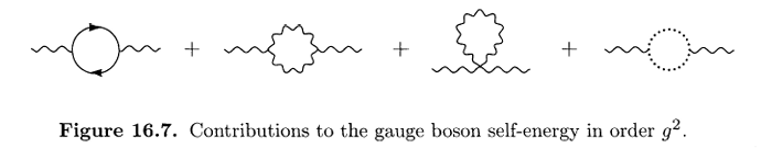
(in addition to these 1PI diagrams, there are three 'tadpole' diagrams; but these automatically banish, as in QED, by the argument given below Eq. (10.5).) The fermion loop diagram can be considered separatetly from the other diagrams, since in principle we could include any number of fermions in the theory. We will see below that the contributions of the three remaining diagrams interlock in an essential way.
Fermion Sector
Let us first calculate the fermion loop diagram. The Feynman rule for the vertices is this diagram is identical to the QED Feynman rule, except for the addition of a group matrix $t^a$ that acts on the fermion gauge group indices. The value of this diagram is therefore the same as in QED, Eq. (7.90), multiplied by a trace over group matrices.

$$=\mbox{tr}[t^at^b]i(q^2g^{\mu\nu}-q^\mu q^\nu)\times \frac{-g^2}{(4\pi)^{d/2}}\int^1_0 dx8x(1-x)\frac{\Gamma(2-\frac{d}{2})}{(m^2-x(1-x)q^2)^{2-d/2}}.$$ The value of the trace is give by Eq. (15.78): $\mbox{tr}[t^at^b]=C(r)\delta^{ab}$. In a theory with several specise of fermions, there would be a diagram of this type for each species. We will be mainly interseted in the divergent part of this diagram, which is independent of the fermion mass. If there are $n_f$ species of fermions, all in the smae representation $r$, then the total contribution of fermion loop diagrams takes the form $$\begin{align} \sum_{\mbox{fermions}} \left( \sim\! \bigcirc\! \sim \right) = i(q^2g^{\mu\nu}-q^\mu q^\nu)\delta^{ab}\left( \frac{-g^2}{(4\pi)^2}\cdot \frac{4}{3}n_f C(r)\Gamma(2-\frac{d}{2})+\cdots\right).\end{align}$$
Pure Gauge Sector 1
Now consider the three diagrams from the pure gauge sector. The contribution of these diagrams depends on the gaug; we will use Feynman-'t Hooft gauge, $\xi=1$.
Using the three-gauge-boson vertex from Fig. 16.1, we can write the first of the fhree diagrams as

$$\begin{align}=\frac{1}{2}\int \frac{d^4p}{(2\pi)^4}\frac{-i}{p^2}\frac{-i}{(p+q)^2}g^2f^{acd}f^{bcd}N^{\mu\nu},\end{align}$$ where the numerator structure is $$N^{\mu\nu}=\left[ g^{\mu\rho}(q-p)^\sigma+g^{\rho\sigma}(2p+q)^\mu+g^{\sigma\mu}(-p-2q)^\rho\right] \times \left[\delta^\nu_\rho(p-q)_\sigma+g_{\rho\sigma}(-2p-q)^\nu+\delta^\nu_\sigma(p+2q)_\rho\right] .$$ The overall factor of $1/2$ is a symmetry factor. The contraction of structure constants can be evaluated using Eq. (15.93): $f^{acd}f^{bcd}=C_2(G)\delta^{ab}$.
To simplify the expression further, combine denominators in the standard way: $$\begin{align}\frac{1}{p^2}\frac{1}{(p+q)^2}=\int_0^1 dx \frac{1}{((1-x)p^2+x(p+q)^2)^2}=\int_0^1 dx \frac{1}{(P^2-\Delta)^2},\end{align}$$ where $P=p+xq$ and $\Delta=-x(1-x)q^2$. Then (60) can be rewritten $$=-\frac{g^2}{2}C_2(G)\delta^{ab}\int_0^1dx\int \frac{d^4P}{(2\pi)^4}\frac{1}{(P^2-\Delta)^2}N^{\mu\nu}.$$ The numerator structure can be simplified by eleminating $p$ in favor of $P$, discarding terms linear in $P^\mu$ (which integrate symmetrically to zero), and replacing $P^\mu P^\nu$ with $g^{\mu\nu}P^2/d$ (also by symmetry): $$N^{\mu\nu}=-g^{\mu\nu}\left[ (2q+p)^2+(q-p)^2\right] - d(q+2p)^\mu (q+2p)^\nu+\left[ (2q+p)^\mu (q+2p)^\nu + (q-p)^\mu (2q+p)^\nu - (q+2p)^\mu(q-p)^\nu + (\mu \leftrightarrow \nu )\right]$$ $$\rightarrow -g^{\mu\nu}P^2 \cdot 6(1-\frac{1}{d})-g^{\mu\nu} q^2 \left[ (2-x)^2 + (1+x)^2 \right] + q^\mu q^\nu \left[ (2-d)(1-2x)^2 + 2(1+x)(2-x)\right].$$
The final step in the evaluation is to Wick-rotate and apply the integration formulae (7.85) and (7.86). This brings the diagram into the following form: $$\begin{align}=\frac{ig^2}{(4\pi)^{d/2}}C_2(G)\delta^{ab}\int_0^1 dx \frac{1}{\Delta^{2-d/2}} \times \left( \Gamma(1-\frac{d}{2})g^{\mu\nu}q^2 \left[ \frac{3}{2}(d-1)x(1-x)\right] \nonumber\\+ \Gamma(2-\frac{d}{2})g^{\mu\nu}q^2 \left[ \frac{1}{2}(2-x)^2+\frac{1}{2}(1+x)^2\right] - \Gamma(2-\frac{d}{2})q^\mu q^\nu \left[ (1-\frac{d}{2})(1-2x)^2+(1+x)(2-x)\right]\right).\end{align}$$
Pure Gauge Sector 2
Next consider the diagram with a four-gauge-boson vertex. Using the vertex Feynman rule in Fig. 16.1, we find

$$\begin{align}=\frac{1}{2}\int \frac{d^4p}{(2\pi)^4}\frac{-ig_{\rho\sigma}}{p^2}\delta^{cd}(-ig^2)\times \left[ f^{abe}f^{cde}(g^{\mu\rho}g^{\nu\sigma}-g^{\mu\sigma}g^{\nu\rho}) \nonumber\\+ f^{ace}f^{bde}(g^{\mu\nu}g^{\rho\sigma}-g^{\mu\sigma}g^{\nu\rho})+f^{ade}f^{bce}(g^{\mu\nu}g^{\rho\sigma}-g^{\mu\rho}g^{\nu\sigma})\right] .\end{align}$$
The factor $1/2$ in the first line is a symmetry factor. The first combination of structure constants in the vertex factor vanishes by antisymmetry; the second and third can be reduced by the use of Eq. (15.93). We then find simply $$\begin{align}=-g^2C_2(G)\delta^{ab}\int\frac{d^4p}{(2\pi)^4}\frac{1}{p^2}\cdot g^{\mu\nu}(d-1).\end{align}$$In dimensional regularization, the integral over $p$ gives a pole ate $d=2$ but yields zero as $d\rightarrow 4$. We could simply discard this diagram and trust that the pole at $d=2$ is canceled by the other two diagrams. It is instructive, however, and no more difficult, to demonstrate the cancellation explicitly. To do so, we can force the integral to look like that of the previous diagram, multiplyiing the integrand by $1$ in the form $(q+p)^2/(q+p)^2$. We then combine denominators as before, and eliminate $p$ in favor of the shifted variable $P=p+xq$. After dropping the term linear in $P$, we obtain $$=-g^2C_2(G)\delta^{ab}\int_0^1dx\int \frac{d^4P}{(2\pi)^4}\frac{1}{(P^2-\Delta)^2}g^{\mu\nu}[P^2+(1-x)^2q^2].$$ We can now Wick-rotate and integrate over $P$ to obtain $$\begin{align}=\frac{ig^2}{(4\pi)^{d/2}}C_2(G)\delta^{ab}\int_0^1dx\frac{1}{\Delta^{2-d/2}}\times \left( -\Gamma (1-\frac{d}{2})g^{\mu\nu}q^2[\frac{1}{2}d(d-1)x(1-x)]-\Gamma(2-\frac{d}{2})g^{\mu\nu}q^2[(d-1)(1-x)^2]\right).\end{align}$$
Pure Gauge Sector 3
Expression (62) and (65), by themselves, do not add to any reasonable value: The pole at $d=2$ does not cancel, and the sum does not have a transverse Lorentz structure. To bring the gauge self-energy into its desired form, we must include the diagram with a ghost loop. According to the rules shown in Fig. 16.5, this diagram is

Sum of Pure Gauge Sector
Now we are ready to put these results together. In the sum of the three diagrams, the coefficient of $\Gamma(1-\frac{d}{2})g^{\mu\nu}q^2x(1-x)$ is $$\begin{align} \frac{1}{2}(3d-3-d^2+d-1)=(1-\frac{d}{2})(d-2).\end{align}$$ The first factor cancels the pole of the gamma function at $d=2$. Thus, the sum of the three diagrams has no quadratic divergenceand no gauge boson mass renormalization. Notice that the ghost diagram plays an essential role in this cancellation.
After the pole at $d=2$ is canceled, $\Gamma(1-\frac{d}{2})$ becomes $\Gamma(2-\frac{d}{2})$. This term therefore combines with the others that are proportional to $\Gamma(2-\frac{d}{2})g^{\mu\nu}q^2$, to give a total coefficient of $$\begin{align} (d-2)x(1-x)+\frac{1}{2}(2-x)^2+\frac{1}{2}(1+x)^2-(d-1)(1-x)^2.\end{align}$$ Since the best way to simplify this expression is not obvious, let us put it aside and work first with the coefficient of $\Gamma(2-\frac{d}{2})q^\mu q^\nu$: $$\begin{align} -(1-\frac{d}{2})(1-2x)^2-(1+x)(2-x)+x(1-x)=-(1-\frac{d}{2})(1-2x)^2-2.\end{align}$$ If the total self-energy is to be proportional to $(g^{\mu\nu}q^2-q^\mu q^\nu)$, it must be possible to reduce expression (69) to this same form (times -1). To do so, note that $\Delta$ is symmetric with respect to $x\leftrightarrow (1-x)$, and therefore we can substitute $(1-x)$ for $x$ in any term of the numerator. In particular, terms that are linear in $x$ can be transformed as follows: $$\begin{align}x\rightarrow \frac{1}{2}x+\frac{1}{2}(1-x)=\frac{1}{2}.\end{align}$$
In the end, the sum of the three pure-gauge diagrams simplifies to $$\begin{align} \frac{ig^2}{(4\pi)^{d/2}}C_2(G)\delta^{ab}\int_0^1dx \frac{\Gamma(2-\frac{d}{2})}{\Delta^{2-d/2}}(g^{\mu\nu}q^2 - q^\mu q^\nu)[(1-\frac{d}{2})(1-2x)^2+2].\end{align}$$ This expression is manifestly transverse, as required by the Ward identity of the non-Abelian gauge theory. For future reference, we record the ultraviolet divergent part of (70):

The $\beta$ Function
The simplest calculation that involves a gague-invariant combination of radiative corrections is the computation of the leading term of the Callan-Symanzik $\beta$ function of a non-Abelian gauge theory. The invariance of the leading term of $\beta$ could be argued intuitively, by saying that the coupling constant of the gague theory should not evolve to large values in one scheme of calculation while it stays small in another scheme. In Section 17.2 we will demonstrate this result more cleanly by showing that the leading coefficient of the $\beta$ function can be extracted from a physical cross section and so must be gague independent. (Surprisingly, this conclusion actually applies to the first two coefficients of the $\beta$ function, written as a power seires in $g$.)

In order for the counterterm $\delta_3$ to cancel the divergence of Eqs. (16.59) and (16.71), it must be of the form $$\begin{align}\delta_3=\frac{g^2}{(4\pi)^2}\frac{\Gamma(2-\frac{d}{2})}{(M^2)^{2-d/2}}\left[ \frac{5}{3}C_2(G)-\frac{4}{3}n_fC_(r)\right],\end{align}$$ where $M$ is the renormalization scale. Depending on the precise renormalization conditions used, there may by additional finite contributions to $\delta_3$, but these do not contribute to the $\beta$ function (to one-loop order). Similarly, the finite parts of $\delta_2$ and $\delta_1$ will depend on the details of the renormalization scheme. However, as we saw in Section 12.2, the one-loop contribution to the $\beta$ function is the same in any scheme is which amplitudes are renormalized at a point where all momentum ijnvariants are of the same order $M^2$. In dimensional regularization, a logarithmic divergence always takes the form $\Gamma(2-\frac{d}{2})/\Delta^{2-d/2}$, where $\Delta$ is some combination of momentum invariants. Thus, to compute the $\beta$ function, we can simply set $\Delta=M^2$ in such expressions.
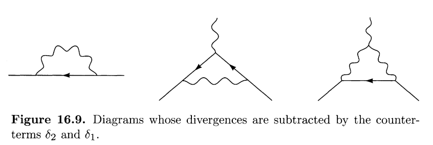
To complete the computation of the $\beta$ function, we must compute $\delta_2$ and $\delta_1$ to the same level of approximation. The fermion self-energy counterterm $\delta_2$ cancels the divergence proportional to $\gamma^\mu k_\mu$ in the first diagram of Fig.16.9. In Feynman-'t Hooft gague, the value of this diagram is
$$\begin{align}=\int \frac{d^4p}{(2\pi)^4}(ig)^2\gamma^\mu t^a \frac{i(\gamma^n p_n + \gamma^m k_m)}{p+k}^2\gamma_\mu t^a \frac{-i}{p^2}.\end{align}$$ Since the divergence in the field strength renormalization is independent of the fermion mass, we have simplified (75) by setting the mass to zero. The product of group matrices equals the quadratic Casimir operator, by definition (15.92). The Dirac matrix structure can be reduced using a contraction identity (7.89). The rest of the calculation follows the same steps as for the boson self-energy diagrams: $$\begin{align}=g^2 C_2(r)(d-2)\int \frac{d^4p}{(2\pi)^4}\frac{(\gamma^n p_n + \gamma^m k_m)}{(p+k)^2p^2}\nonumber\\ =g^2C_2(r)(d-2)\int_0^1dx\int\frac{d^4P}{(2\pi)^4}\frac{(1-x)\gamma^n k_n}{(P^2-\Delta)^2}\nonumber\\ =\frac{ig^2}{(4\pi)^{d/2}}C_2(r)\gamma^n k_n \int_0^1 dx(1-x)(d-2)\frac{\Gamma(2-\frac{d}{2})}{\Delta^{2-d/2}}\nonumber\\ =\frac{ig^2}{(4\pi)^2}\gamma^n k_n C_2(r)\Gamma(2-\frac{d}{2})+\cdots.\end{align}$$ (Here $P=p+xk$ and $\Delta=-x(1-x)k^2$.)
The divergent part of this expression must be canceled by the second counterterm diagram of Fig. 16.8. Thus, if the renormalization scale is $M$, the counterterm must be $$\begin{align} \delta_2=-\frac{g^2}{(4\pi)^2}\frac{\Gamma(2-\frac{d}{2})}{(M^2)^{2-d/2}}\cdot C_2(r),\end{align}$$ plus finite terms. We note that, like $\delta_3$, $\delta_2$ depends on the gauge; for example, $\delta_2$ has no one-loop divergence in Landau gague ($\xi=0$).
To determine $\delta_1$, we must compute the second and third diagrams of Fig. 16.9. The second diagram, computed in Feynman-'t Hooft gague and for massless fermions, is

$$\begin{align}=\int \frac{d^4p}{(2\pi)^4}g^3t^bt^at^b\frac{\gamma^\nu ((/p)+(/k'))\gamma^\mu((/p)+(/k))\gamma_\nu}{(p+k')^2(p+k)^2p^2}.\end{align}$$ The gauge group matrices can be simplified according to $$\begin{align} t^bt^at^b=t^bt^bt^a+t^b[t^a,t^b]=C_2(r)t^2+it^bf^{abc}t^c\nonumber\\ =C_2(r)t^a+\frac{1}{2}if^{abc}\cdot if^{bcd}t^d=[C_2(r)-\frac{1}{2}C_2(G)]t^a.\end{align}$$ In the third line we have used the antisymmetry of $f^{abc}$ to rewrite the matrix product as a commutator; in the last line we have used Eq. (15.93).
The diagrams compted earlier in this section had positice superficial degrees of divergence, so we needed to extract their logarithmic divergences carefully. The integral in (78), however, is superficially logarithmically divergent, and so the coefficient of this divergence can be extracted easily by considering the limit in which the integration variable $p$ is much greater than any external momentum. In this limit, the diagram is estimated as follows: $$\begin{align}\sim g^3[C_2(r)-\frac{1}{2}C_2(G)]t^a \int \frac{d^4p}{(2\pi)^4}\frac{\gamma^\nu /p \gamma^\mu /p \gamma_\nu}{p^2\cdot p^2\cdot p^2}.\end{align}$$ If we replace $p^\rho p^\sigma$ by $g^{\rho\sigma}p^2/2$ is the numerator of (80), this expression simplifies easily: $$\begin{align}\sim [C_2(r)-\frac{1}{2}C_2(G)]t^a(2-d)^2\frac{1}{d}\gamma^\mu \int \frac{d^4p}{(2\pi)^4}\frac{1}{(p^2)^2}\nonumber\\ \sim\frac{ig^3}{(4\pi)^2}[C_2(r)-\frac{1}{2}C_2(G)]t^a\gamma^\mu (\Gamma(2-\frac{d}{2})+\cdots).\end{align}$$ This estimate gives the correct coefficient of the divergent term. It drops completely the finite terms in the vertex function, but we do not need these to compute the $\beta$ function.
The third diagram of Fig. 16.9 can be analyzed in the same way. Its value, in Feynman-'t Hooft gague and for massless fermions, is

$$\begin{align} =\int \frac{d^4p}{(2\pi)^4}(ig\gamma_\nu t^b)\frac{i(/p)}{p^2}(ig\gamma_\rho t^c)\frac{-i}{(k'-p)^2}\frac{-i}{(k-p)^2}\nonumber\\ \times gf^{abc}\left[ g^{\mu\nu}(2k'-k-p)^\rho + g^{\nu\rho}(-k'-k+2p)^\mu+g^{\rho\mu}(2k-k'-p)^\nu\right].\end{align}$$ The gauge matrix product can be reduced as follows: $$f^{abc}t^bt^c=\frac{1}{2}f^{abc}t^d=\frac{i}{2}C_2(G)t^a.$$ Again we can determine the logarithmic divergence of this diagram by neglecting all external momenta in comparison with $p$. A straightforward calculation then yields $$\begin{align} \sim \frac{g^3}{2}C_2(G)t^a\int \frac{d^4p}{(2\pi)^4}\gamma_\nu (/p) \gamma_\rho \frac{g^{\mu\nu}p^\rho-2g^{\nu\rho}p^\mu+g^{\rho\mu}p^\nu}{(p^2)^3}\nonumber\\ \sim \frac{g^3}{2}C_2(G)t^a\frac{1}{d}\int \frac{d^4p}{(2\pi)^4}\frac{1}{(p^2)^2}\left[ \gamma^\mu \gamma^\rho \gamma_\rho - 2\gamma^\rho\gamma^\mu\gamma_\rho+\gamma^\sigma\gamma_\sigma\gamma^\mu\right] \nonumber\\ \sim \frac{ig^3}{(4\pi)^2}\frac{3}{2}C_2(G)t^a\gamma^\mu (\Gamma(2-\frac{d}{2})+\cdots).\end{align}$$ In the second line we have again replaced $p^\rho p^\sigma$ with $g^{\rho\sigma}p^2/d$.
The sum of the divergences in results (81) and (83) must be canceled by the third counterterm diagram in Fig 16.8. With a renormalization scale of $M$, we find $$\begin{align}\delta_1=-\frac{g^2}{(4\pi)^2}\frac{\Gamma(2-\frac{d}{2})}{(M^2)^{2-d/2}}[C_2(r)+C_2(G)].\end{align}$$ Notice that $\delta_1$ is not equal to $\delta_2$, as would have been true in the Abelian case: here $\delta_1$ has an extra term, proportional to $C_2(G)$.
We are now ready to compute the $\beta$ function. Plugging the three counterterms (74), (77), and (84) into our formula (73), we find $$\beta(g)=(-2)\frac{g^3}{(4\pi)^2}\left[ (C_2(r)+C_2(G))-C_2(r)+\frac{1}{2}\left( \frac{5}{3}C_2(G)-\frac{4}{3}n_fC(r)\right)\right];$$ that is, $$\begin{align}\beta(g)=-\frac{g^3}{(4\pi)^2}\left[ \frac{11}{3}C_2(G)-\frac{4}{3}n_fC(r)\right].\end{align}$$ Notice that, at least for small values of $n_f$, the $\beta$ function is negative and so non-Abelian gauge theories are asymptotically free. This is a resulf of exceptional physical importance,first discovered by 't Hooft, Polizer, and Gross and Wilczek. We will discuss the physical interpretation of this resulf turther in Section 16.7, and in the next several chapters. However, for the rest of this section, we will resist the temptation to pursue the physics and instead complete out technical analysis of the divergences of non-Abelian gauge theoreis.
Realtions among Counterterms
16.6. Asymptotic Freedom: The Background Field Method
Background Field Perturbation Theory
One-Loop Correction to the Effective Action
Computation of the Functional Determinants
16.7 Asymptotic Freedom: A Qualitative Explanation
Reference
Peskin - An Introductin To Quantum Field Theory Chapter 16